pigeon background: the frequency domain 🕊️

I figured that it may be worth a quick crash course on IQ samples, the time domain and the frequency domain. I have written a bit about processing IQ data from SDRs previously, which may be a helpful reference point to start with if this is entirely new, but if that all makes sense, I figured I’d do a base-level orientation to keep the pigeon series as self-contained as I can.

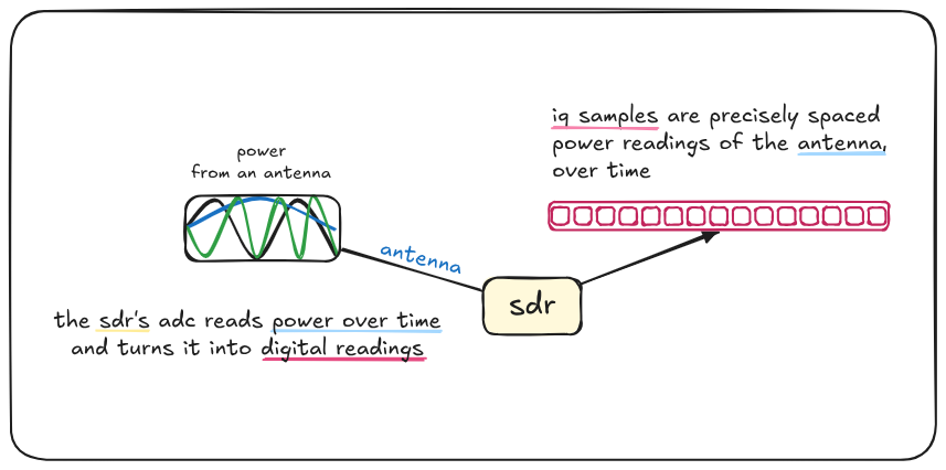
However, the only thing you really need to keep in mind about iq samples (“time domain” iq samples like we get from an SDR) to start is that they are precisely spaced power readings of an antenna, over time. Each sample represents the power observed from the antenna at a specific instant. Fundamentally, this is no different than using the GPIO pin to read an analog value in a for loop and sending those values back to a computer, except the the numbers wind up being complex, rather than scalar, power values.

Without getting too far into the why, the only meaningful point here is that we need to use complex numbers due to the practical nature of processing data at such high frequencies. Generally speaking (there are always exceptions), the signal leaving (or going into) your RF front end hardware on the PCB will be in the form of two traces – one for I (“in-phase”) and one for Q (sampled 90 degrees out of phase from “I”) – sampling both at the same instant gives you a complex number (power reading from the antenna at that very instant).

It may be tempting to shed yourself of this perceived numerical shackle as quickly as possible, however, turning that back into a scalar number for your DSP code to use (It works for audio, why not RF!) genuinely looses enough information along the way that it’s just plain easier to work with the complex numbers all the way until you’re able to extract a scalar signal from your complex number stream, like we did with PACKRAT.

Once we have IQ, we can do all sorts of fun things to our stream in the time domain (things like like filtering them, turning them into AM or FM audio streams, all sorts of stuff!) – but the real fun happens when we use a FFT to measure the frequencies that make up our window of time-domain samples. We can process the frequency-domain data to our hearts content, and optionally, pair our frequency domain adventures with an iFFT to generate time-domain samples that are comprised of the desired frequency components that we can transmit over the air.

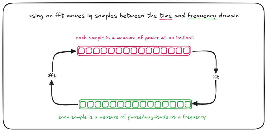
Each “bin” in the frequency domain represents the average amount of power and average phase offset at a specific frequency, over the duration of the time-domain samples provided.

I’ve always looked at frequency-domain bins and seen the keys of a piano. Each key, when pressed, has its own distinct frequency. You can press a key very softly or strike a key with intent (fortissimo!) to change how loud the frequency is (the “magnitude”). You can press many keys at the same time and you hear those frequencies at the same time – a chord. This, conceptually, is all the “inverse FFT” (iFFT) is doing. We’re going from frequency inputs (keys pressed) to an audio stream (sound waves). Unfortunately, an FFT has no similar analogy in my head – but to tourture this metaphor even further for the one musician out there still reading – think of it like a player piano that makes no noise, but when it hears a specific note, the keys will press themselves down by how strong that note is. This special player piano, when it hears a G7♯9 played next to it – will press the G, B, D, F, and A♯ keys without making a noise.

The maximum and minimum observable frequency in the frequency domain is determined by the sampling rate in the time domain. The relationship between observable frequency and sampling rate is called the nyquist frequency.

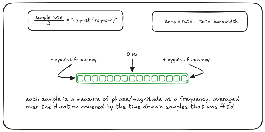
The number of time-domain samples and frequency-domain bins match 1:1 - 64 time domain samples in result in 64 frequency domain bins out of a fft. As a result, increasing the number of samples the fft operates over increases the frequency domain “resolution”, not observable frequencies (each “bin” represents an increasingly narrow slice of frequency), at the expense of time-domain resolution (each bin now represents an average over a longer amount of time).

The Frequency Domain is also a handy way to do a few specific (and expensive) time-domain operations – for instance, when computing cross-correlation or convolution, the time domain operation is very expensive – but using the frequency-domain allows this operation to be done through “mere” multiplication.

In-memory Layout

OK the diagram above was a bit of a lie. In-memory fft frequency domain bins don’t usually go from negative to positive. The native layout of a FFT is generally what I’ve called “Zero First”, where the first frequency bin is 0 Hz, followed by bins increasing in frequency until the Nyquist frequency bin, followed by the negative Nyquist frequency bin up in frequency back to just below 0 Hz.

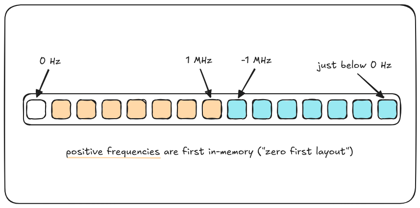
However, I write things out for human consumption (and things like subcarrier plans) in what I call “Negative First” order, where the first bin is the most negative Nyquist frequency bin, up to 0 Hz, and then up to the positive Nyquist frequency bin.

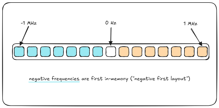
I find that this is the layout that most humans expect frequency domain data in, for example, with waterfall plots. This layout means the frequency domain window has no “jumps” in frequency, and visually inspecting it is a lot easier. As evidenced by my diagrams above, when I am working with frequency domain data (as a person, not as a programmer), I find it a lot easier to shift to a Negative First ordering.

Let’s talk about the phy →