finding the needle in a haystack (Part 5/12) 🕊️

I’ve found the most important factor to demodulation is getting timing right. Timing is incredibly important. Being off by a sample can cause incredible amounts of corruption and can easily result in the total loss of a Burst. This means that we care a great deal about when exactly a burst starts, and finding a way to detect that with some degree of reliability. This turns out to be a particularly hard problem, and one that requires the cooperation of the sender and receiver to work.

I opted to use a very well understood and widely adopted algorithm usually referred to as “Schmidl-Cox”, written up in the December 1997 paper entitled Robust Frequency and Timing Synchronization for OFDM by Timothy M. Schmidl and Donald C. Cox. This technique relies on the presence of a preamble with a specific predefined periodic structure, at a specific sample rate and duration. This repeating structure turns out to be uncommon enough in noise that it can be exploited to extract the specific sample at which a Symbol (such as an OFDM Symbol) begins in the Time Domain.

Throughout the Schmidl-Cox paper, the cyclic nature of a preamble is referred to as L, the number of IQ samples between each repeating segment. A preamble that is 128 samples long, repeating twice (two segments of 64 samples) means the L value is 64.

The Schmidl-Cox algorithm is, effectively, a filter which responds to a strong signal which repeats every L samples. The Schmidl-Cox detector is the place where I’ve spent the most time (by far) on Pigeon, and it’s also one place where I’m least confident that it’s behaving as expected (although it has been behaving lately).

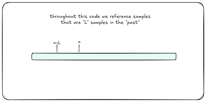
While implementing the filter, a common pattern I’ve adopted from others that came before me is to go “back in time” by L samples when generating metrics.

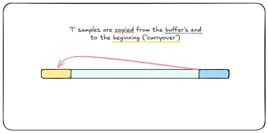
As you may have guessed by now, since we operate on fixed-size windows of incoming data rather than a stream, we need some way to retain L of each metric from the end of the last window for the next batch of IQ samples (r) that passes through. I decided to solve this by implementing what I have called internally a “carryover buffer” to hold all of the Schmidl-Cox internal metrics. The purpose here is to always maintain a “carryover” of L samples at the beginning of the buffer which are the final L samples from the last run of the detector to the beginning of the buffer (“carryover region”).

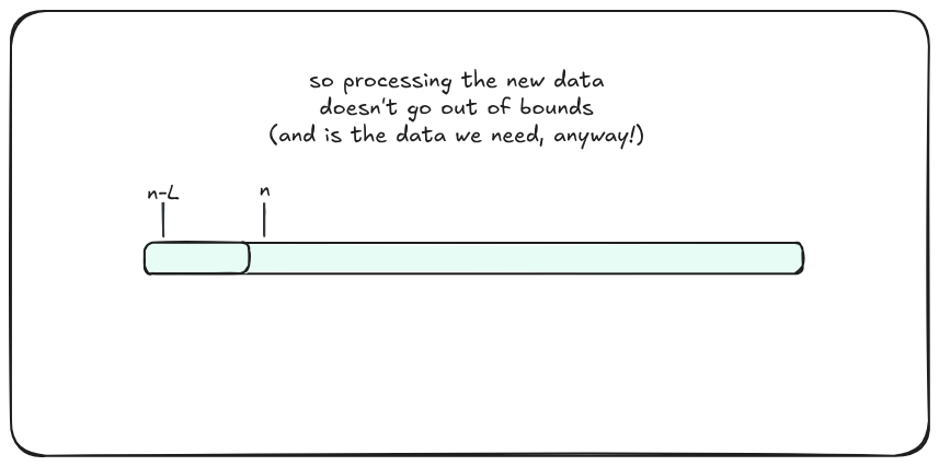
When we get new data (new iq samples from our SDR, called r in the paper), we ensure the “caryover” is copied to the front of the list, and write (or compute) the new data, starting L samples into the buffer (“new region”).

This makes our code happy, and allows the Schmidl-Cox internal buffer size be any length and the computed metrics will always match any other sized detector operating over the same data (and there’s test coverage to prove it!)

There’s a bunch of metrics that make up the Schmidl-Cox filter – we’ll get into them later – but each of the Schmidl-Cox metrics gets its own “carryover buffer”, which are kept in sync any time new IQ samples (r) are provided to the detector.

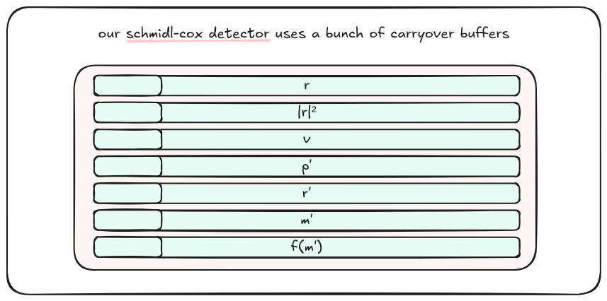
This collection of carryover buffers and computed metrics is what I’ve been calling the “Detector” – we use the detector by writing complex valued IQ samples to it, and we get back the scanner detection metric m'.

/// Schmidl-Cox detector state.
pub struct Detector { ... }

impl Detector {
    /// Compute the Schmidl-Cox 'M' autocorrelation metric.
    pub fn compute_m(&mut self, buf_in: &[IQ]) -> &[f32] {
        ...
    }
}

I opted to return a borrow against the internal m' carryover buffer, which reduced copies at the expense of some lifecycle headaches during debugging.

Schmidl-Cox

The Schmidl-Cox metric (M) is, at a high level, a measure of of how much power (R) is measured over how “L-cyclical” the signal is (P). As the signal gets stronger and the signal gets more “cyclical”, the metric goes up. Conversely, if the signal is not very cyclical, or not strong, the metric will remain low.

The original Schmidl-Cox paper defines some variables that, for the sake of clarity, i’m going to keep the same throughout my code. It’s helpful when working back and forth between the paper and the code – so let’s do that here too. The only trouble is in a few places there are uppercase variables such as r vs R, which I (lightly) edited to be r and r_prime, respectively.

However, if you look close, these variables will still be slightly different than the actual paper. Namely, I’ve taken advantage of the same shortcuts as the DSP Illustrations series – they’ve all been reworked to only use IQ samples that came before it, rather than samples that come after. This, along with some careful math, means these metrics can be implemented as FIR filters, which is easier (computationally) than the many inner for loops as-written in the paper. This has two big implications – first is, as I’ve mentioned above, we’re always looking back by L samples into the past, and second, that we’re going to have a time delay between the M metric and the iq samples (r).

Let’s jump into actually computing this stuff.

The first metric we can compute is v – a measure of how similar each IQ sample is to a sample L symbols ago.

Just to state it explicitly (since it’s otherwise implicit in my LaTeX notes) the multiplication here is complex multiplication, using the complex conjugate. Let’s go ahead and implement generating the v metric off the incoming iq (r):

  for (v, r_last, r_now) in self.buf_v[working_window]
      .iter_mut()
      .zip(
          self.buf_r[last_l_window]
              .iter()
              .zip(&self.buf_r[working_window].iter()),
      )
      .map(|(out, (i1, i2))| (out, i1, i2))
  {
      *v = *r_last * r_now.conj();
  }

Next up is not a part of the paper – it’s never explicitly computed in the paper – but there’s a lot of places where we use the phasor’s magnitude squared, so let’s just do that once for every input sample r and write it out to r_sq.

If you think of this as an (x, y) point, the magnitude becomes the hypotenuse, and using magnitude squared instead of magnitude directly means we can avoid the (more expensive) sqrt call, turning this into, fairly simply, (iq.real * iq.real) + (iq.imag * iq.imag) (what I call abs_square).

  // precompute r_mag_square to avoid recomputing it
  for (r_mag_square, r) in self.buf_r_mag_square[working_window]
      .iter_mut()
      .zip(self.buf_r[working_window].iter())
  {
      *r_mag_square = r.abs_square();
  }

With r_sq and v out of the way, we can use both to compute the R (or r') metric – which is a measure of power, over a window of L samples long.

The tricky bit here is we have an edge-case that will fail using our FIR-based approach – so to properly bootstrap R, for the 0th value, we’ll need to compute it in the way the Schmidl-Cox paper describes. This R initialization is pretty straightforward – we need to add up a bunch of power measurements to get the baseline for the FIR filter state. We can implement by adding up L samples-worth of r_sq values, so that we have a “prior” state at the 0th element.

A bit of sum should do the trick:

  self.buf_r_prime[start] =
    buf_r_mag_square[start..start + self.l]
        .iter()
        .sum();

Since the initial state is computed, we can now use prior R state to keep the FIR filter running – think of this as a set of FIR filter taps all set to 1, where we can “simply” add the new sample and subtract the sample that just “fell off” to generate the filter output, lather, rinse, repeat.

Which we can go ahead and implement:

  let mut r_prime = &mut self.buf_r_prime[working_window];
  let r_prime_it = r_prime.iter_stride_mut(
    StrideOffset::Forward(1)).zip(
        self.buf_r_mag_square[working_window]
          .iter()
          .zip(
            self.buf_r_mag_square[last_l_window].iter()),
  );

  for (
      (r_prime_last, r_prime_now),
      (r_mag_square_now, r_mag_square_last)
  ) in r_prime_it {
      *r_prime_now =
          (*r_prime_last
            + *r_mag_square_now
            - *r_mag_square_last)
          + f32::EPSILON;
  }

Some of y’all keen readers may be wondering what iter_stride_mut does – it’s a bit of (admittedly unsafe-using) rust which allows me to iterate over a slice, taking a borrow on &mut T and a &T separated by some fixed non-zero span. The implementation of that is pretty boring, but it’s a handy little trait for times like this.

Next metric we need to generate is our P metric, which is a filter for how L-periodic the signal is, which we can compute by making yet another FIR-like filter over v.

We can now use the same iter_stride_mut technique to build up the P filter with something like this:

  let mut p_prime = &mut self.buf_p_prime[working_window];
  let p_prime_it = p_prime.iter_stride_mut(StrideOffset::Forward(1)).zip(
      self.buf_v[working_window]
          .iter()
          .zip(self.buf_v[last_l_window].iter()),
  );

  for ((p_prime_last, p_prime_now), (v_now, v_last)) in p_prime_it.zip(r_prime_it) {
      *p_prime_now = *p_prime_last + *v_now - *v_last;
  }

Finally, we can compute the final Schmidl-Cox M metric by putting P over R (How periodic is the signal over the strength of the signal)

Which turns into a fairly boring bit of division:

  for (m_prime, r_prime, p_prime) in slice_zip2_mut(
      &mut self.buf_m_prime[working_window],
      &self.buf_r_prime[working_window],
      &self.buf_p_prime[working_window],
  ) {
      // r is always greater than 0 thanks to the EPSILON offset
      // above, otherwise, we can wind up getting REALLY small which
      // spikes the metric.
      *m_prime = p_prime.abs_square() / (*r_prime * *r_prime);
  }

And there we have it! The M metric that we can work off of. Let’s take a look into what we’re expecting things to look like.

oll korrect?

I wasn’t kidding earlier – this bit of code is easily, and by far the place where i’ve spent the most time on Pigeon. This has been an absolute onslaught of bugs – and worse yet – bugs often still result in a usable output metric!

It’s incredibly easy for a deep and systemic bug to last for months, get wrapped up into an abstraction layer, and silently introduce bugs at the edge of what you can test for. To help others along, I figure I should post a few simulated plots of the Schmidl-Cox metric to help with visually debugging the M metric output.

Up first, let’s take a look at the M metric for a high SNR (low noise) burst. I’ve put a Pigeon burst through an AGWN channel, passed that resulting IQ stream into the detector, and charted the M metric over the beginning of the burst.

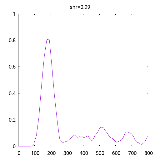
You can see something pretty distinctive in there – the metric stays low, spikes high, forms a bit of a plateau, and then drops back down. The plateau is dependent on how many IQ samples are within the L-periodic window, usually it’s L less than the preamble length.

The output Schmidl-Cox metric values are also fairly sensitive to noise, even though detections will still be detectable well past when the OFDM signal is recoverable (at least for me, and now). We can see this when we take the same chart as above, except sweep from a high SNR to a fairly low SNR:

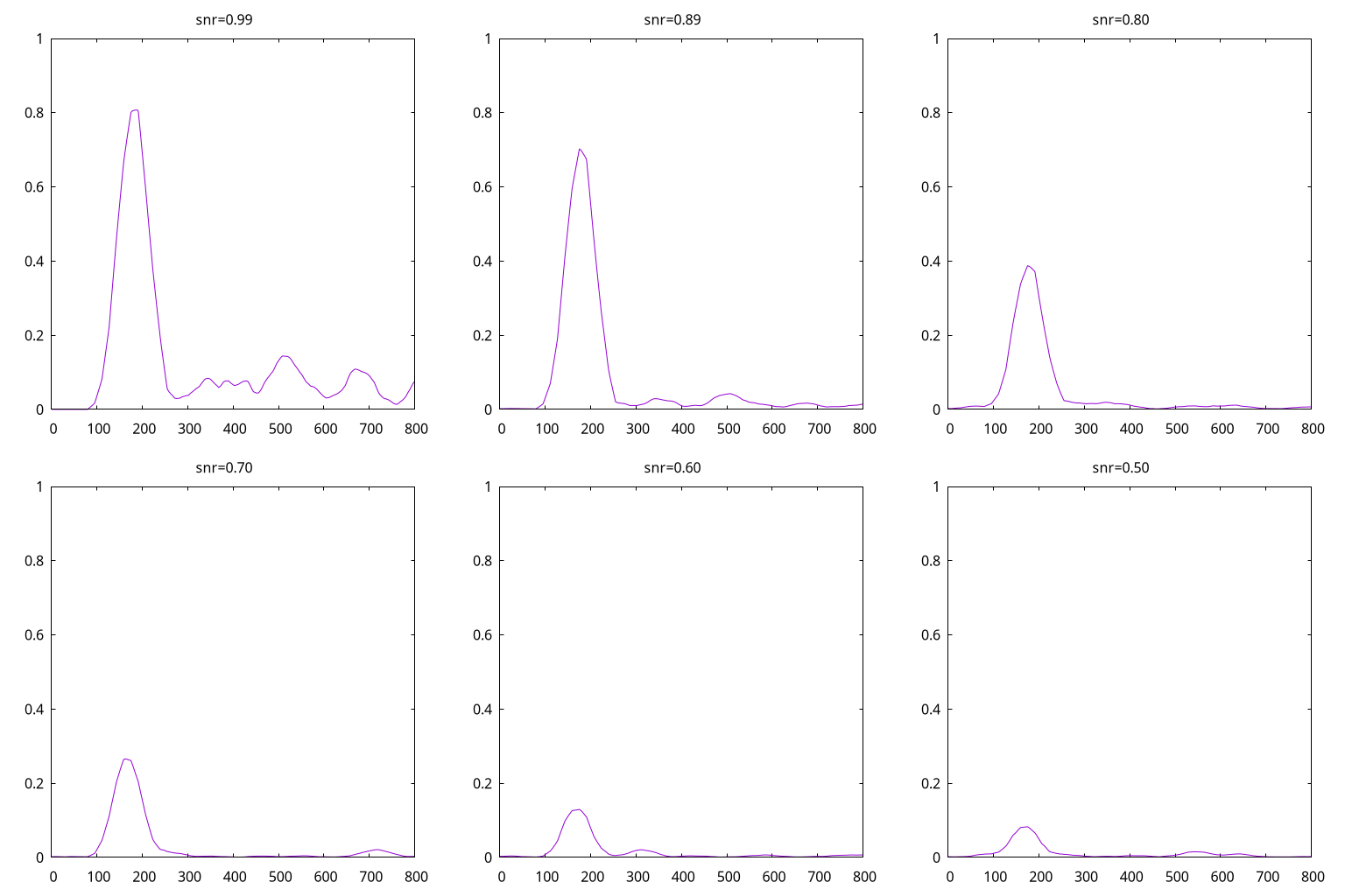
This means that when we do attempt to find a detection, we’ll need to trigger based not on some absolute threshold, but rather, some relative metric. I wound up settling on some code that’s a bit hacky but has worked well enough for now which searches for the m metric raising above some threshold (threshold), searching for the first peek of the m metric (over a maximum distance of horizon) within the provided m metric buffer.

// (lightly edited for clarity)

/// Search through the schmidl-cox M metric and identify the
/// most likely start to a burst.
fn search(
  threshold: f32,
  horizon: usize,
  m: &[f32]
) -> Vec<(usize, f32, f32)> {
    let mut ret = Vec::new();
    let mut m_iter = m.iter().enumerate();

    // rough outline of the approach here is to scan through
    // the 'm' metric until we get to something past our
    // threshold. After we find the likely starting spot,
    // we'll scan the iterator forward to the `horizon`.

    while let Some((idx, v)) = m_iter.next() {
      if *v > threshold {

        // the `m` metric is over the threshold value provided.
        // that means we should now find the peek in the m
        // metric to determine where our starting point is.

        // rather than consume the iterator, we're going to
        // re-borrow the `m` metric into `m_search`.
        let m_search = &m[idx..(idx + horizon).min(m.len())];
        if m_search.is_empty() {
          continue;
        }

        // next up is that we're going to scan through the
        // `m_search` slice and find where `m` goes from
        // increasing to decreasing (trailing edge).

        let mut idx_sync = 0;
        let mut m = *v;
        for (idx, (v_last, v_now)) in m_search
            .iter()
            .zip(m_search[1..].iter())
            .enumerate()
        {
          if v_now - v_last < 0.0 {
            m = *v_last;
            idx_sync = idx;
            break;
          }
        }

        // after we have our best-guess start location
        // (idx + idx_sync), we can put together our
        // detection, append it to our return values,
        // and advance the iterator past our horizon.

        let snr = m / threshold;
        ret.push((
          idx + idx_sync,
          m,
          snr,
        ));

        // consume the iterator past the horizon
        for _ in 0..horizon {
          m_iter.next();
        }
      }
    }

    ret
}

This, of course, now begs the question regarding what a sensible threshold value should be, or even, just like, how to find one.

Detection Thresholds

Fairly early on I wrote a very basic simulator, which I used to rough in some arbitrary constants. They also made for some pretty cool images, so I’m going to subject you, dear reader, to them as well. Each of these images was generated by “sending” and “receiving” Pigeon frames through a simulated channel (with added AGWN, etc).

To help illustrate what is going on when picking a threshold, I generated an image where each pixel is a simulated run of 16 trials each, at each schmidl-cox detection threshold (x-axis) for a given simulated SNR (y-axis). This graph shows a measure of if the packet(s) transmitted were successfully demodulated (regardless of spurious detections!) As you might expect, as the Schmidl-Cox detection threshold is raised (going down on the y-axis), the higher the SNR needs to be (going right on the x-axis).

Ideally, you’d want to pick a threshold which is based on the signal to noise ratio, and have it be high enough to not trigger too much (missing packets), but also not having it so low that we spend all our time attempting to demodulate every single IQ index as its own burst.

It was hard to find a lot out there about this – supring because it seems like such an important topic. Given the m metric very subjective (two radios next to each other can have wildly different values depending on when they turned on first) – I just kinda YOLO’d this part.

I wound up defining my absolute threshold value (as passed into search above) as being derived from the average m value – my threshold value of 1 would be “anything at or above the average m metric, while 1.5 would be “anything 1.5 times the rolling m average value”. The m_avg is computed by using a filter update value (m_avg_beta) to use the average of each window computed to update the rolling average.

Tuning all of this has been a headache, but it’s been a lot less of a headache than trying to use constant thresholds. I suspect I will invest some time in the future running a bunch of simulations to see if there’s anything I can learn here.

Using the Scanner

Now that we have a working detector, we can wrap that up inside something that I’ve called a Scanner. I debated if I should collapse the Detector and the Scanner into a single construct, but opted not to due to the number of issues I’ve had with the Detector – test coverage became more important to me than a clean abstraction and a bit of conceptual duplication. While the Detector can search over IQ samples and return us the M metric, the Scanner is a higher-order construct responsible for scanning over incoming IQ values, returning windows of just the IQ samples thought to contain Bursts.

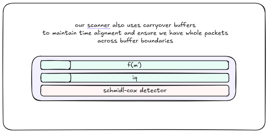
Similar to the Detector, our Scanner also holds two “carryover buffers” for the m metric and iq data, which are sized a lot larger – enough to hold multiple bursts – as well as the Detector that it is wrapping.

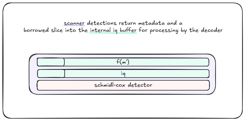
Let’s get to work, let’s go ahead and call the detector to compute our m metric (as well as the m_avg, which we update the rolling average state for) and return our “ScanDetection“s – blocks of IQ suspected to contain a Burst.

// (lightly edited for clarity)

impl FrameScanner {
  ..

  /// Scan over an incoming buffer, computing M
  fn scan(&mut self, buf: &[IQ]) -> Vec<ScanDetection<'_>> {

    // call the `Detector` to compute the Schmidl-Cox
    // `M` metric.
    let (m_avg, m) = self.detector.compute_m(buf);

    // implement carryover of m and iq to handle
    // burst split across iq buffer bounds
    self.copy_tail_to_head();

    // update the current m metric average
    self.update_m_avg(m_avg);

    // get borrows to the m metric aligned
    // to the iq buffer.
    let m = self.m();
    let iq = self.iq();

    // compute what our m metric threshold is based
    // on tuned constants and the average m value
    let threshold = self.threshold();

    let mut ret = vec![];
    for detection in search(
      threshold,
      self.mode.preamble.samples(),
      m
    ) {
      let ( idx, m, snr ) = detection;

      // compute the range of iq that the burst
      // is contained in
      let range = idx..(idx + self.mode.samples());

      // and a borrow of the underlying iq
      // buffer for the detection
      let snippit = &iq[range.clone()];

      ret.push(ScanDetection {
        m,
        range,
        snippit,
        snr,
      });
    }

    ret
  }
}

As you may have noticed, we return a borrow of the underlying iq carryover buffer – we can avoid a bunch of copies by doing this. The downside is, of course, that we need to fully process all the ScanDetection objects before we can take out a mutable copy of the internals again – which can be a bit annoying when extracting underlying detector state in tests.

Let’s talk about estimating what happened to the packet in transit →