Pow! QAM-o! Bam! (Part 2/12) 🕊️
Paul Tagliamonte 2026-09-08 diyIf you're looking for it, the intro to the PHY (layer 1) that this belongs at a high level and listing of the parts that make it up (including this one) is on the phy post.
I find the most pesky part of sending digital data over rf is the act of mapping bits of information to some measurable rf property. You want to cram as much as you can in there but still make it so that a noisy signal is well understood. At the lowest possible level, this is all our subcarrier modulation schemes are doing – taking bits in, and producing some signal state that we will transmit over the air. Modulation is a tricky topic worth exntensive decades-long research and development – and I fully intend to do exactly that – playing with modulation schemes sounds incredibly fun. To start, though, I want to be sure that known, well-understood and boring choices work, so that’s where we’re going to live here – boring, well-understood choices.
Although this section is perhaps definitely absolutely definitely maybe out of order, we’re going to start here. We start here not just because it’s where I started when I got started on the PHY (it was) – but because the next post is going to assume a base level of knowledge about how this all works and I’m trying to avoid turning this series into a goosebumps novel.
Before we begin, it bears repeating: I plan to experiment (and change!)
modulation schemes within pigeon after this is all working well. In order to
enable that very experimentation, I was sure to make the process of modulating
and demodulating bits and IQ something I could swap out. I settled on a trait
(for non-rustaceans out there – that’s fine, none of the code here will be
very rust-y – for our purposes here today, a trait is basically the same
thing as an interface in Go or Java) that looks like this:
/// Convert data into IQ subcarriers and vice versa.
trait Modulation {
    /// Number of bits we can store in an IQ sample using this
    /// modulation scheme.
    const BITS_PER_SYMBOL: usize;

    /// Modulate the input bits into the output frequency
    /// domain bins, returning the number of bins set.
    fn modulate(dst: &mut [IQ], src: &bit::Vector) -> usize;

    /// Demodulate the input frequency domain bins into the
    /// output bits, returning the number of bits set.
    fn demodulate(dst: &mut bit::Vector, src: &[IQ]) -> usize;
}
Since I wanted to avoid hard-coding QPSK everywhere, I’ve implemented and
tested with two schemes to start with – QPSK, and QAM-16. The pigeon test
suite runs against both of them, keeping these codepaths exercised. Although
both can reasonably be called “QAM” (I mean sure why not, QAM-4 is just
QPSK), I still have a tendency to use QPSK since I started with BPSK.
Just in case I slip up (or it reads as confsuing) – QAM-4 and QPSK are
the same thing. Heck, I’d even go so far as to say QAM-2 and BPSK are
the same thing, too!
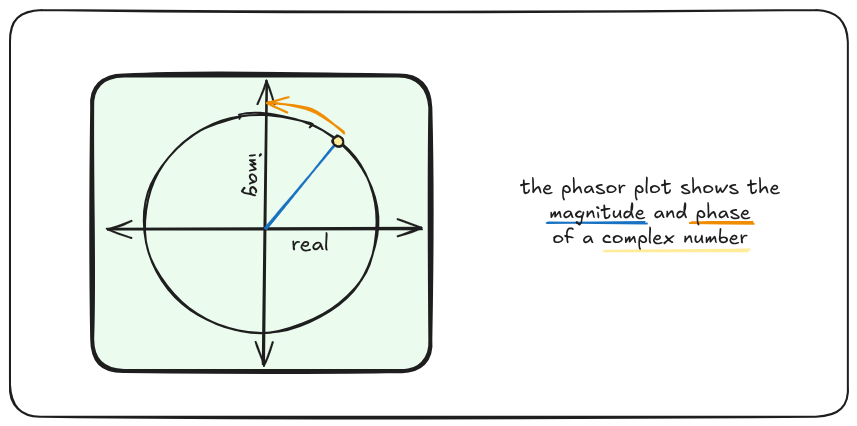
When we talk about modulating subcarriers in pigeon, we’re talking about
working with a frequency domain bin of
phase and magnitude, which we will manipulate to encode data. Traditionally,
we plot that value in a
phasor diagram,
where we plot the real and imaginary scalar components of the complex
number like x and y points on a chart. We can freely convert between
thinking of this like x/y style real/imag scatter plot, or a
r/θ style phase/magnitude polar plot.
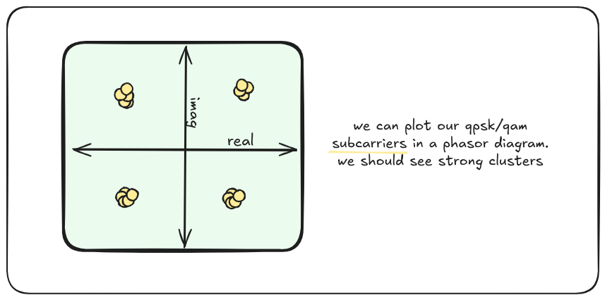
If all goes well with our transmission and receiving process – plotting
QAM/BPSK/QPSK points on a Phasor Diagram should show tight clusters of
plotted points centered around the “constellation” points, each of which
represent a different bit pattern being sent or received.
QPSK
QPSK is where a carrier wave
signal is modulated between 4 different phase states 90° apart. In the same way
PACKRAT uses BPSK to shift between two phase states
(in-phase and 180° (or one-half 𝜏) out of phase) – QPSK shifts between four
phase states, each (90° (or one-quarter 𝜏)) out of phase from each other,
something like 1+1j, -1+1j, -1-1j and 1-1j. Using QPSK, we can transmit
2 bits per symbol with QPSK rather than 1 bit with BPSK.
QAM-16
QAM-16 is a technique
where a carrier wave is modulated in both phase and amplitude, such that the
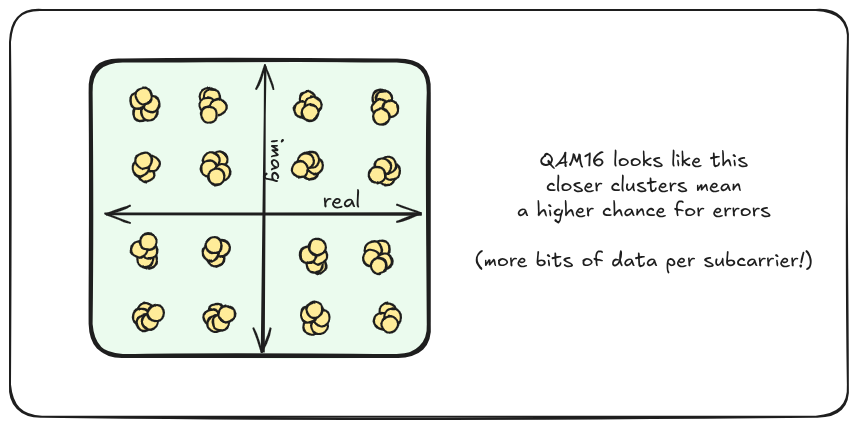
frequency domain complex vector is shifted between 16 points (in a 4 x 4 grid).
Conceptually, this becomes a bit more clear if the phasor real and imag
values are treated as cartesian x and y coordinates, moving between 16
fixed points on a 4 x 4 grid between +1 and -1 This scheme allows 4 bits
to be transmitted per symbol.
Creating and decoding QAM points is a bit of an art, but it’s also fairly
straightforward to take a naive approach and get fairly far with it. Each QAM
constellation point can be thought of as being on a grid, separated by a fixed
distance (determined by the number of points in the constellation – or the
“order” – to evenly spread each point along the odd numbered “rows” and
“columns”). This may not be one’s instinct for implementing QPSK (seems
a lot simpler to just use the real/imag scalar value sign data to read/write
2 bits of information and call it a day) but it’s hard to not contend with
this reality for QAM-16 and above.
Similarly, during demodulation, each point can be compared against the even numbered points along the “rows” and “columns” to determine the best matching location for the IQ sample. You could imagine comparing the euclidean distance from a subcarrier to each constellation point and finding the nearest neighbor – or, more simply for our grid layout – split the plot up into 4 or 16 grid squares and determine which contains our point.
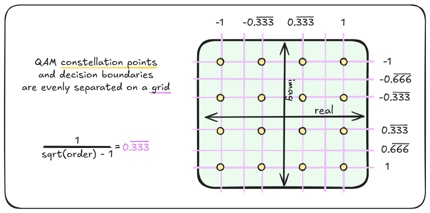
As an example, with an order of 16, each point on our grid will be
separated by 0.333..., placing each encoded constellation point along the
real and imaginary axis at the (odd numbered) points: -3*0.333...,
-1*0.333..., 1*0.333..., and 3*0.333.... On the other end, when
we’re trying to determine what point a sample represents, we can (for
conceptual illustration here) brute force compare to see which evenly spaced
points contain us (-4*0.333... > iq > -2*0.333...,
-2*0.333... > iq > 0*0.333..., …) to our sample – or, more simply –
divide the point by our grid spacing (0.333...) with a max/min bound.
As for how to map the bits to QAM constellation points – this, too, is a bit
of an art. I opted to start with the easiest thing I could, which is to split
the bit range into two, and use the low and high half of the value to index
into the constellation by row and column. There’s all sorts of better
techniques out there – things like using
gray code to ensure adjacent bins
are only a single-bit flip off (rather than what I’ve done, where noise that
bumps QAM subcarriers from one of the two center columns will flip a 01 to
10 – two bits different. I’m planning to spend a lot of time on my QAM code
in the future – so hopefully more trip reports to come in the future.
Encoding QAM/QPSK
Since I realized I could be lazy and implement both QPSK and QAM-4 using
the same code but with a const passed in (as a generic) for the constellation
size, I decided to do exactly that. Laziness always prevails. First let’s
sketch out our Qam struct, and have it take a generic argument (a constant
usize numerical value, not a type) which indicates the constellation’s
size.
#[derive(Debug, Copy, Clone)]
pub struct Qam<const ORDER: usize>;
In the future, when I go to swap out the Constellation layout like
non-uniform constellations or the underlying bit mapping technique, I want
to be able to swap out the existing technique without doing a bunch of work.
I implemented the rectangular QAM constellation layout (what we’ll do in this
post) within a helper struct named Grid. When I go to revisit this code, my
plan is to pull Grid out of the Qam implementation and make that
a generic argument to Qam as well. Let’s implement Grid, which has
all our interesting implementation logic.
/// QAM Constellation of some power of two order (4, 16, 32)
#[derive(Debug, Copy, Clone)]
pub struct Grid<const ORDER: usize>;

/// When we set a value to 1+1j, we're actually
/// outside the unit circle. Here we're going to
/// instead set a maximum point of 0.707+0.707,
/// so that the magnitude is never greater than
/// 1.0.
const ONE: f32 = 0.707;

impl<const ORDER: usize> Grid<ORDER> {
  /// ORDER_I is the number of points on a single
  /// side of the QAM constellation.
  const ORDER_I: usize = ORDER.isqrt();

  /// ORDER_I2 is the number of points that are
  /// either positive or negative within the
  /// constellation.
  const ORDER_I2: usize = Self::ORDER_I / 2;

  /// GRID_V is the spacing and furthest
  /// extent of our QAM constellation.
  const GRID_V: f32 = 2.0
    / ((Self::ORDER_I as f32 * 2.0) - 2.0)
    * ONE;

  /// Bitmask used to split our u16 input bits
  /// into points on the real (and imag) axis.
  const MASK: u16 = (1 << Self::ORDER_I2) - 1;

  /// Take some input bits, and modulate those
  /// bits into a point on the QAM constellation.
  fn data_to_iq(d: u16) -> IQ {

    // Here we're going to mask the incoming bits (`d`)
    // into the lower bits (which will be modulated to
    // control the `real` axis), and the higher bits
    // (`imag` axis).

    IQ::new(
      Self::data_to_scalar(d & Self::MASK),
      Self::data_to_scalar(
        (d >> Self::ORDER_I2) & Self::MASK
      ),
    )
  }

  /// Take some input IQ point, and demodulate that
  /// point back into bits.
  fn iq_to_data(iq: IQ) -> u16 {

    // Here we're going to take a guess for both the real
    // and imag axis, and set those into the high and
    // low bits.

    Self::scalar_to_data(iq.real)
        | (Self::scalar_to_data(iq.imag) << Self::ORDER_I2)
  }

  /// Take our input and determine which X or Y point to use
  /// based on the input value.
  fn data_to_scalar(d: u16) -> f32 {

    // Map the input bits from 0->N (where N is dictated by the
    // QAM order) to -1 to +1.
    let position = ((d as f32 * 2.0) + 1.0)
        - (Self::ORDER_I as f32);

    position * Self::GRID_V
  }

  /// Take some scalar X or Y point, and determine what the
  /// original bits must have been.
  fn scalar_to_data(s: f32) -> u16 {

    // Map the input scalar from -1 to +1 to 0->N (where N is
    // dictated by the QAM order).
    let position = ((s / Self::GRID_V) - 1.0) / 2.0;

    (position + (Self::ORDER_I2 as f32)).round() as u16
  }
}
As for actually using Grid within Qam to satisfy our Modulation
interface, the next step is to implement the Modulation trait (again,
non-rust people: just read this as “interface” in this context and you’ll be OK)
for Qam by using our Grid helpers above.
impl<const ORDER: usize> Modulation for Qam<ORDER> {

  // The number of bits we can store is the same as our
  // 'ORDER_I' constant in the grid -- the square root of
  // the qam constellation size.
  const BITS_PER_SYMBOL: usize = Grid::<ORDER>::ORDER_I;

  fn modulate(dst: &mut [IQ], src: &bit::Vector) -> usize {

    // First, we will figure out how many IQ samples we
    // will need.

    let iq_len = src.len() / Self::BITS_PER_SYMBOL;

    // Now, for each IQ sample, extract a window of input
    // bits, and set the IQ sample to that modulated point.
    //
    // This will give us a flat buffer of modulated
    // frequency-domain IQ samples, which we can use later
    // on.

    for (idx, dst) in dst[0..iq_len].iter_mut().enumerate() {
      let idx = idx * Self::BITS_PER_SYMBOL;
      let bits = src.slice(idx, idx + Self::BITS_PER_SYMBOL).as_u64();
      *dst = Grid::<ORDER>::data_to_iq(bits as u16);
    }

    iq_len
  }

  fn demodulate(dst: &mut bit::Vector, src: &[IQ]) -> usize {

    // Determine how many bits we will need.
    let bit_len = src.len() * Self::BITS_PER_SYMBOL;

    // Now, for each IQ sample, demodulate the
    // constellation point into bits, and set those
    // bits in the destination buffer.

    for (idx, src) in src.iter().enumerate() {
      let idx = idx * Self::BITS_PER_SYMBOL;
      let mut b = bit::Vector::from_bytes(
        &Grid::<ORDER>::iq_to_data(*src).to_le_bytes()
      );
      b.resize(Self::BITS_PER_SYMBOL);
      dst.set_range(idx, idx + Self::BITS_PER_SYMBOL, &b);
    }

    bit_len
  }
}
Tidy. That should be easy enough to fix when I get back to it in the future. Since I’m a visual person – I figured this is a great spot to help illustrate how this QAM code will map bits to IQ points on a phasor diagram. I wrote a small program to generate a phasor diagram and modulating the bit pattern from 0 to 15 using a QAM-16 constellation as described above. I also added a bit of noise so the points weren’t all stacked on top of each other, in case you’re wondering why they’re not all the same point.

Speaking of noise, it’s also a good time to get into the last set of things to know about the pigeon modulation scheme – this whole process is just super sensitive to even slight errors. I’ve had to learn about (and fix) a seemingly never-ending stream of failure modes – and correcting the QAM subcarriers yields massive performance returns.
I’m going to outline a few of the common failure modes I’ve had to contend with here and how I identify them by eye.
Clock Errors (so many)
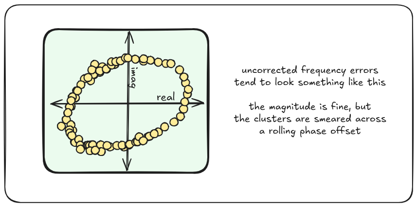
There’s just so many ways this stuff can break because clocks don’t all agree on what a “second” is – like that’s even a thing we can define anyway. Two oscillators being off by some fixed amount, or an oscillator changing in frequency (like an OCXO warming up) all falls into this category. In general though, one of the most common ways I’ve seen clocks cause errors with QAM is easily spotted when the constellation winds up smearing into a circle – usually a sign that there’s some uncorrected frequency difference. The fix here is usually to get better about frequency correction or channel estimation (we’ll get into that in upcoming posts).
Noise Errors
Like most other digital protocols, QAM is fairly sensitive to noise. Usually
we’d call just regular “noise” AGWN, or “Additive Gaussian White Noise”. As
the noise goes up, the constellation gets more diffuse. As AGWN gets stronger
compared to the signal, the white noise will induce phase and and magnitude
errors that get bigger and bigger. To illustrate what happens to our
constellation as noise increases, I ran pigeon packets through a simulated
channel and plotted the demodulated constellation while increasing the AGWN
for each generated plot:
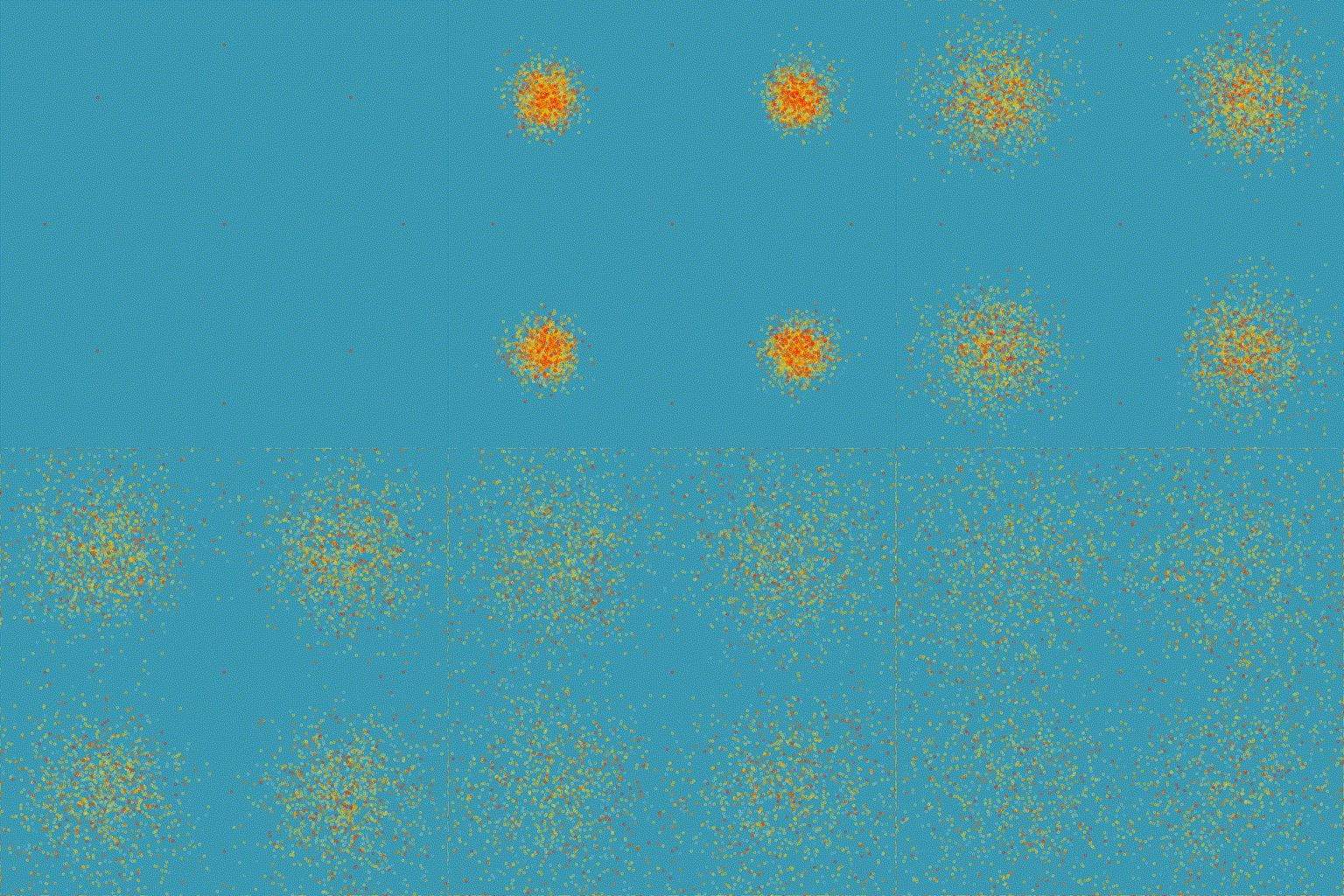
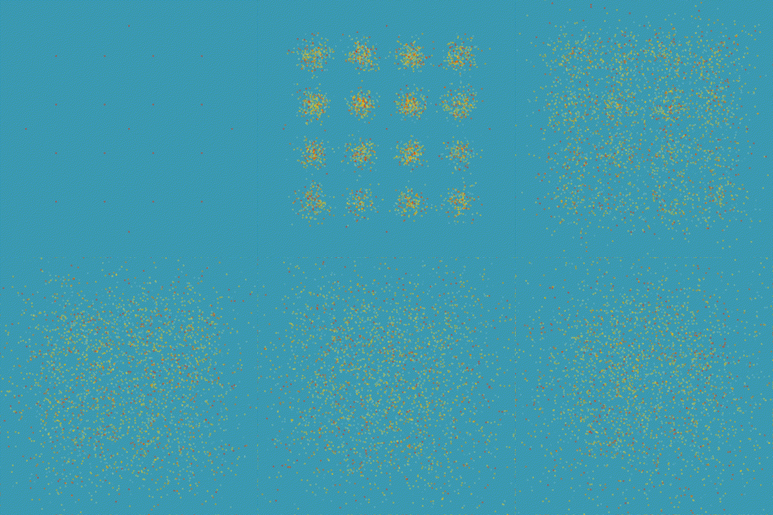
The signal hangs on for a lot longer than you might expect – but winds up bleeding into neighboring constellation bins pretty quickly. As the QAM constellation gets more dense, AGWN becomes more and more of an issue. I ran the same simulation as above, but this time using QAM-16. Let’s take a look at what that looks like:
The line between signal and noise is incredibly fragile – the more work we can put into ensuring a good, well understood and clean channel, the better. Even something as simple as missing a detection peek by a few samples can completely crash the decoder. Here’s a plot of the decoded QAM subcarriers, inducing a delay from 32 samples early to 32 samples late. You can see how quickly the constellation snaps into focus (mostly because the frequency offset estimation and pilot-based channel estimation correction kicks in), then turns into noise again.
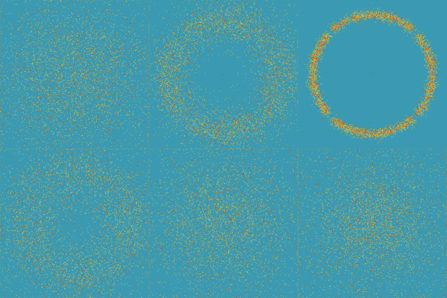
It may feel like the amount of time we see tight clusters of QAM data was short,
it’s perhaps underscoring just how tight short that was. The entire duration
of the signal before the constellation snaps into focus was 32 samples. 32
samples, for pigeon (2.5 MHz sampling rate), can be converted back into
seconds. Let’s do that – how long, exactly, is half of this GIF?
12.8 microseconds – being off by around 13 microseconds ether early or late will render the signal undecodable – nevermind the duration of time where the signal is even properly corrected. This is enough of an issue that we’ll go over how to handle detecting pigeon bursts with that level of accuracy in a later post. And all that is only at 2.5 Msps! The casual level of accuracy required here still remains absolutely wild to me. Every cell phone and wifi card kicking around in a junk drawer is capable of that level of accuracy for hours on end.
Data “Whitening”
Although it shouldn’t really matter, in practice, it turns out having a bunch of adjacent frequency domain bins with the same amplitude and phase cause artifacts on demodulation. Fixing this is actually kinda tricky, so I decided to mostly mitigate it by bastardizing a technique called “whitening” (a term derived from white noise – specifically AGWN (as seen just above!). The goal is to make the structured (and mostly set to zero) data look more like random noise in order to spread data out across all the QAM constellation points, in order to avoid artifacts when the signal is sent or received “lopsided”.
Pigeon’s implementation of whitening is to use a well-known and documented
coefficient to seed an
LCG.
You may remember these from C’s rand(3) – something that has generally
fallen out of favor due to the ease of misuse in a setting where you actually
require a
CSRNG,
not just “pseudo-randomized” numbers. I picked an LCG because it’s incredibly
easy to implement, can (deterministically) generate an unbounded amount of
data, and is well understood and documented. LCG works by multiplying (and
incrementing) the seed, modulus m, updating the seed to the “random” output
of the function.
Within Pigeon, our seeded LCG is used to generate as many bytes as are required
in order to stretch that seed into a bit vector of the same length as the PHY
burst, and XOR the PHY burst data with the whitening vector. This means
our LCG implementation is designed to produce an unbounded amount of data,
mostly in the form of iterators that look a lot like:
struct Lcg {
    seed: u32,
    m: u32,
    mult: u32,
    inc: u32,
}

impl Iterator for Lcg {
    type Item = u32;

    fn next(&mut self) -> Option<u32> {
        let mut seed = self.seed;
        let mult = self.mult;
        let inc = self.inc;
        let m = self.m;

        let m_s = std::num::Wrapping(mult)
            * std::num::Wrapping(seed);

        seed = (m_s
            + std::num::Wrapping(inc)).0 % m;

        self.seed = seed;
        Some(seed)
    }
}
I implemented the LCG using u32 (32 bit unsigned integers) to give the
greatest chance of successfully using an off-the-shelf rand implementation;
and since it’s easy enough to implement either way, it’s kinda no big deal if
not. As for the rest of the scheme – in particular, the m, multiplier and
inc fields are the same throughout all pigeon modes, and match what glibc
uses (see earlier rationale; being able to use rand(3) off the shelf would
be nice).
| Attribute | Value | Description |
| m | 0x80000000 | as seen in glibc, (2 to the 31st power) |
| multiplier | 1103515245 | as seen in glibc |
| inc | 12345 | as seen in glibc |
| seed | each mode specifies a unique the seed value |
Even with this whitening process, it is still very possible to generate
pathological payloads which XOR to a long run of the the same value – but
fancier fixes are hard. Given I am (currently) the only user of pigeon, if a
user was to do this, it would be, by definition intentional and fully
coordinated by all parties anyway.
One final note in case there are any readers getting itchy while reading this – although this kinda looks like a “cryptography 101, week 1, day 1” style one-time-pad, it’s worth remembering that this is not actually encryption – even if it was (it’s not), it’s not even something that will run afoul of the FCC rules (“shall not be encoded for the purpose of obscuring their meaning”), since this process both serves a specific engineering purpose at a technical level for the PHY (whitening the data), and the inputs to generate the whitening vector are documented with everything else about this protocol. It’s intended to be widely known by design – and definitely not something who’s purpose or even use is designed to obscure the message contents.